Category: Tech Notes

Download PDF

Many piece-picking systems use tilt tray, Bombay or other types of article sorters to process orders. This paper describes an example of a very low capitalization cost order fulfillment “pull” system using a tilt tray sorter for filling of piece picked orders. The system is based on the design model of “Quick Access Residual Storage (QARS)” (see IIE Solutions May 1997). An interesting feature of this system is the absence of conveyance systems. The system is controlled by the Mandate® AWMS™.

At the heart of the system is a 640-drop station, single induction zone tilt tray sorter. Each of the drop stations has an active order accumulation queue and a packing shelf. The order accumulation queue is separated from the packing shelf by a gate, which is automatically activated by Mandate to release a completed order into the packing shelf as necessary.

The induction zone consists of five SOFT™ purpose-built manual induction stations controlled by Mandate. Product is delivered to induction stations in both full cartons and in “residual” totes uniquely identified by license plate number (LPN).

Most of the product is stored in the bulk stock area. All product in this area is in full cartons. This area is serviced by Mandate equipped Crown SP3000 Stock Selectors for both put-away and retrieval of stock for order fulfillment. The area has both full pallet storage locations and loose individual carton storage shelves. Product is randomly stored (not in fixed locations) in this area. Mandate tracks the stock location of all cartons in this area. Residual stock is that stock which is “left over” after a full carton is opened and its needed product used to fill in-process orders. The QARS model attempts to have only one residual container per SKU.

The residual stock is held in one of two areas. One area is for stock that is not needed for immediately foreseeable orders (“No Near Need” area). This area must have at least enough locations to hold one tote for each SKU. The other area is used for temporarily holding the stock that will shortly be needed for new orders. This area is called the “Near Need” area. This application does not “classify” stock into fast or slow mover categories. Mandate dynamically determines the best area to hold the residual stock based on future order needs. The “No Near Need” totes are stacked on a pallet for random put away into a case rack storage location by a stock picking (also known as cherry picker) vehicle. The “Near Need” area totes are equipped with an inexpensive battery powered OnSite Paging Systems “Container Pager” (patent pending).

The “Near Need” totes are placed on shelves very near the sorter induction stations until Mandate “pages” the tote. This tote is then removed by the worker for re-delivery to sorter induction. The Container Pager has a high intensity light that indicates to the worker the tote is being paged. There is no need to scan totes for either put-away or retrieval in this area.

Operational Flow Overview

Mandate receives ASN (advanced ship notice) information for inbound cartons. Upon receiving trailer arrival, cartons are unloaded and sample audited for shipment integrity. Individual cartons are loaded onto mixed SKU pallets for put-away. The Mandate AWMS allows operational procedures to control the put-away process wherein receipt acknowledgement may occur as the result of unloading the trailer, inspection of goods, loading onto pallets for put-away, or the actual put-away itself. Mandate tracks the location of all product and reports stock positions to an external financial system.

Mandate receives customer orders from a Web enabled order entry and processing entry system. Mandate responds to the order processing system with an “order acceptance” confirmation and an “order shipped” notification. Orders are maintained by Mandate for processing based on the order ship date and priority received from the order processing system.

A “Pending Order” queue is maintained by Mandate. Mandate selects the highest priority shippable orders that will soon be picked and puts them into this queue. This application uses a virtual wave in operating the sorter. A “virtual wave” is defined as a wave where, as existing orders complete and are released from the drop station to the packing shelf, new orders are removed from the “Pending Order” queue and assigned to the newly available drop station.

The Mandate AWMS selects stock to fill orders. The rules for making stock selections are first to empty any residual totes containing needed stock. If there is insufficient residual stock for completing orders, additional needed stock is selected from the full carton storage area. Stock is selected for the orders that are both actively picking and that are in the “Pending Order” queue. Mandate directs the retrieval of selected stock, sequencing the selection to maximize the completion of orders.

Mandate directly controls the induction process itself and the use of an AWMS allows the induction process to be handled independently from the stock selection and delivery process. The induction process is only concerned about filling orders and has no concern from whence the stock came. Any stock delivered to the station will be examined to determine if it could be used to fill orders. If so, Mandate will direct the workstation operator to induct product until either there is no longer a need for the product or the container is emptied. Of course Mandate tracks stock usage. These features allow stock to be manually and independently retrieved from a trailer in the inbound yard and delivered to the sorter induction station. The AWMS adapts to the situation, by updating the receiving system indicating the carton had been received, recording the carton was at the sorter induction, and then completing any orders requiring the stock and updating the carton contents to indicate any remaining stock

Once a carton or tote is no longer currently needed (completed or emptied) at the sorter induction station, it is delivered to an area called “Tote Induction”. Mandate directs the work in this area through Symbol Technologies Model 1700 Palm Based terminals. Empty cartons are put on a chute down to the packing area for shipping use. Empty totes are removed and stacked and any “Container Pager” removed. Cartons with remaining product are scanned into an empty tote. Full totes are scanned for their routing disposition, either to “Near Need” or the “No Near Need” area. If the tote is to be sent to the “No Near Need” area any “Container Pager” is removed. If the tote is to be sent to the “Near Need” area, and if there is an available “Container Pager”, the “Container Pager” is scanned linking it to the tote.

The sorter packing stations are serviced by purpose built SOFT™ mobile pack services stations controlled by Mandate. Workers are directed to orders ready for packing. The mobile pack service stations contain packing cartons, packing material, and shipping label printers. Once cartons are packed and labeled they are stacked on the floor where another worker gathers and delivers them to shipping for sample audit and trailer loading.

Download PDF

Just a few years ago distribution centers handled most of their goods either by a pallet load or as individual closed cases. Piece picking, an operation that demands a lot of resources, was an exception to this rule or was a very small portion of the distribution center operation.

Conditions have changed greatly in recent years. Distribution centers servicing retailers are facing radical changes in ordering patterns. Most retailers have adopted just-in-time inventory practices sustained by smaller, more frequent orders with line item quantities smaller than full case quantities. As companies venture into e-commerce applications, they find that their new Internet customers order mainly single items or—even harder to fulfill—multi-SKU, single-item orders.

Below are several low capital expenditure options available for eight piece-picking operations. The effect of each option is quantified on a pure piece-picking or e-commerce application.

For the purpose of this analysis, the time thatpickers spend in a piece-picking process is divided into three categories: walking between transactions; executing picking transactions (including finding the location to pick from, retrieving requested quantity, placing items in shipping container, and other sub-tasks); and setting up orders (releasing complete orders and starting new orders).

Many piece-picking techniques focus on picking orders in batches in order to reduce the walking between transactions. In highly automated processes (piece sorters, ASRSs) the size of these batches can be very large (more than 2,000 orders) and walking between transactions can almost be completely eliminated. However, these systems require very large initial investments, which are not considered in this analysis.

The costs provided are equipment only and exclude any software costs that may be required to support the option.

The sample application

The piece-picking reference requirements used to compare different technologies are:

• 150 orders per hour with an average of five lines per order and 1.5 items per line
• 12,000 active SKUs to be picked from a combination of flow rack and static rack. The total aisle length adds up to 2,000 feet. The SKUs are small enough to be handled manually by workers.
• The average number of pieces in a receiving case is 20.
• The 80-20 rule applies in this reference application; therefore, 80 percent of the line transactions include the 20 percent most active SKUs (fast movers). Also, the 5 percent most active SKUs (super fast movers) account for 50 percent of the line transactions.
• The distribution center operates two shifts five days per week.

A link to a spreadsheet for people to check the calculations behind the results presented in this document can be found in the conclusions section at the end of the article.

The time parameters used to estimate picking times in each option are walking time per foot, transaction time per line, and setup time per container.

When possible, the best way to estimate these parameters is using software logs of the actual operation and videotape of the operation corresponding to the logs. While the log records provide large data samples already in electronic format, the videotape is very helpful to explain log records that show unexpected deviations from other records of the same tasks. People may question the time parameters used, but even though it may be is easy to disagree with estimations, it is not so easy to disagree with electronic records and videotapes. While the numbers presented here are estimations, they should be representative of a true physical system.

Scenario 1: Individual order picking with paper lists

This is the least sophisticated option to analyze. It implies an operator picking one order at a time from a paper list and having to walk the entire picking loop, meaning the total length of all the picking aisles, to complete the order. This is a very inefficient operation with very low productivity, yielding a high incidence of errors. It will be used only as a base for comparisons. The calculations are performed by the spreadsheet for all the presented scenarios.

To determine productivity and labor:

Lines to pick per loop = 5.0 lines per container X 1 container per loop = 5 lines per loop

Setup time per loop = 5.0 seconds per container X 1 container per loop = 5 seconds per loop

Walking time per loop = 2,000 feet per loop X 0.5 seconds per foot = 1,000 seconds per loop

Transactions time per loop = 5.0 lines per loop X 12 seconds per line = 60 seconds per loop

Total time per loop = 5.0 seconds per loop + 1,000 seconds per loop + 60 seconds per loop = 1,065 seconds per loop

Results

Productivity = 3,600 X 5 / 1,065 seconds per loop = 16.9 lines per hour per picker.
Labor = 150 X 5 X 2 / 16.9 = 88.8 pickers.

Scenario 2: Batch picking with paper lists

This option introduces a picking cart that allows the picking of six orders in the same loop using a paper-picking list. In this scenario the walking time per foot increases because the picker is pushing a cart with six containers on it. The transaction time per line increases because the picker needs to find the container for the picked items among the six on the cart. This option represents a substantial labor reduction with a very low investment in equipment ($300 to $500 per cart); however, it does not address the problem with errors.

Productivity = 67.0 lines per hour per picker. Labor = 22.5 pickers.

Scenario 3: Batch picking with handheld scanner terminals

This option eliminates all paper from the operation by replacing paper lists with handheld terminals. These terminals are capable of task validation through the scanning of picked items and destination containers. The transaction time per line and the setup time per container increase because pickers have to scan items and containers in this scenario.
The labor reduction with this option is still very substantial and the errors are almost completely eliminated with the validation. The required investment in equipment is in the range of $1,500 to $2,000 per handheld terminal plus the communication system.

Productivity = 64.0 lines per hour per picker. Labor = 23.4 pickers.

The original handheld terminals tied one hand of the picker completely. Manufacturers of these devices have developed units that pickers can carry attached to their wrist or finger, partially returning the use of the two hands to the pickers.

Voice terminals that issue verbal picking commands and accept verbal responses from pickers can replace the handheld terminals. Voice technology leaves workers’ hands completely free for picking and excels in transactions that require heavier than usual data exchange between the software and the worker, such as exceptions handling. On the other hand, without a scanner, validations become more cumbersome as workers need to read data on labels back to the software. Voice technology is an option that can be very attractive for some applications.

Scenario 4: Batch picking with smart carts

Handheld terminals have small displays that limit the amount of information available to the picker. A smart picking cart furnished with an onboard computer and with one or more full-size monitors can become a very powerful source of information for the picker: current location of the cart highlighted in an aisle layout, optimal or shortest route to the next picking location, next bay location to pick from highlighted in a graphical bay layout, bin location identification to pick from, full description of item to pick, quantity to pick, picture of item to pick, etc. The required time per transaction can be reduced with a carefully designed system presenting useful information to the picker.

Increasing the batch size from one to six orders results in a large productivity increase; however, further increases in the batch size could be limited by other factors such as carton size and/or the weight of the picking cart in a manually pushed cart operation. A self-propelled smart cart could be considered to eliminate some of these restrictions.
This option introduces smart carts into the operation. The batch size increases from six orders to 12 orders per loop. Walking time per foot increases because the picking cart is larger. Transaction time per line increases because the picker needs to sort the picked items to 12 containers instead of to 6.

Smart carts can bring an even larger labor reduction, the same accuracy as with handheld terminals, and a sophisticated interface traveling with the picker providing all information necessary for the picking tasks. Smart carts with the features mentioned should be in the $10,000 to $15,000 per cart range.

Productivity = 89.0 lines per hour per picker. Labor = 16.9 pickers.

Scenario 5: Virtual batching with smart carts

Many people dislike an inherent fact linked to batch picking: Containers that have been completed still have to be carried on the cart until the completion of the picking loop. This situation is particularly undesirable when the picking loop is very long and the number of picks per container is low. The condition is even worse when orders require more than one container per order and all the containers are carried the full length of the picking loop.

The most efficient solution for this issue is the use of virtual or dynamic batching. When an order is completed, the software can inform the picker that the container does not have any more pending picks, allowing the picker to release that container and start a new one. The released container can be dropped on the aisle or moved to a top shelf in the cart — a shelf not ergonomically useful for picking. The top shelf can also be used to carry empty containers. Once the cart goes by a point where it can release containers, like a take-away conveyor spur, all containers on the top shelf can be released. The concept of a single build cart area in the loop disappears and is replaced by a continuous loop that has neither an end nor a beginning.

The impact to productivity comes from the reduction in the actual walk required to complete a container. Defining the virtual loop length as the expected distance walked to complete a container, its value would be the total actual length of the picking loop multiplied by two factors.

Virtual loop length = Actual loop length X (N/(N + 1)) X (1/M)

In the equation, N is the average number of lines per container and M is the average number of containers per order.

The expected effect of this option in our application is below. The setup time per container increases because containers are now released in two steps. This option yields a labor reduction of 9 percent that can be achieved without any additional investment in equipment. The only potential investment is in software to support it.

Productivity = 97.0 lines per hour per picker. Labor = 15.4 pickers.

Fast moving – slow moving separation

The intelligent selection of picking locations for each individual SKU (slotting) also has an impact on DC productivity. Among several slotting strategies, fast moving SKUs can be segregated from the other SKUS and picked with a different process that better fits their requirements. Fast mover SKUs and slow mover SKUs behave differently from the picking perspective. For fast movers there is shorter walking distance between transactions, the bulk of the picking time is in the actual picking task. Conversely, for slow movers there is longer walking distance between transactions. This results in the walking time being the largest component of the picking time for slow movers.

Scenario 6: Pick fast movers with pick-to-light and slow movers with smart carts

This option separates the 5 percent fastest moving SKUs that account for 50 percent of the transactions and place them in a pick-to-light aisle. Pick-to-light is an option that can reduce by more than half the transaction time per line. The length of this aisle is 120 feet. The other SKUs (slow movers) are picked with smart carts.

The pick-to-light aisle will need to be split in sections with one picker working each section in a pick and pass process. There is no batch picking in this aisle.

This particular application does not seem to benefit from pick-to-light; nevertheless, this technology is very attractive for high density picking applications. The cost of pick-to-light technology is in the range of $125 to $175 per SKU location.

Scenario 7: Pick fast movers with smart carts and slow movers with carousels

An available technology that addresses the excessive walking in slow moving zones is carousels. Carousel pods substantially reduce the long walking between picks for slow movers. The picker does not need to go to the location; instead the location comes to the picker. As the picker is completing a transaction other carousels in the pod are rotating to be ready for the picker by the time he completes the current transaction, reducing picker idle time between transactions. Productivity using this type of device can easily reach 250 lines per hour per picker.

This option separates the 20 percent fastest moving SKUs, which account for 80 percent of the line transactions activity, to process them with smart carts. The length of these fast moving aisles is 400 feet. The other 9,600 SKU (slow movers) are picked from a carousel pod.

Even though the calculations show a very attractive labor reduction, the problem with this particular application is to have all the required inventory of 9,600 SKUs in one carousel pod. Carousel technology in this case addresses very well the throughput requirements but not the storage requirements. The cost of carousel technology is in the range of $350,000 to $500,000 per carousel pod. With this cost, this option could be considered a borderline low capital expenditure option.

Scenario 8: Pick fast movers with smart carts and slow movers with a two-step picking process

Another option to deal with the excessive walking in slow moving zones is two-step picking. Smart carts picking in slow moving zones could be picking larger batches than 12 orders per loop. For instance, workers could be picking to six containers. Each of these containers, instead of representing a single order, could represent all the items required by the 12 orders in a smart cart picking in the fast moving zones. The items in each container would be mixed together in this first step. After the cart is finished, the slow moving cart would be parked in the path of the fast moving cart. The picker of the fast moving cart would stop in front of the container and do a second sort from the slow moving cart single container to his six individual order containers. Walking between picks is reduced at the price of touching twice the slow moving items.

This option keeps the 20 percent fastest moving SKUs to process them with fast moving smart carts. These carts also do the second sort of the items coming from the slow moving zones. The length of these aisles is 432 feet. These 2,400 SKUs account for 80 percent of the transactions.

Smart carts carrying six containers pick the other slow moving SKUs. Each of these six containers collects the items for 12 orders picked as a batch in the fast moving zone. The slow moving aisles add up to 1,600 feet.

The calculation shows that even with the additional step for picking slow movers, this option offers an increase in total productivity of the system. The only additional investment would be more floor space in the fast moving area to park the smart carts coming from the slow moving zone. Of course, the software would need to support this operation, which requires the pre-picking of the items in the slow moving zones and directing the fast moving carts to the locations where the pre-picked items are. This option also can be implemented pre-picking items from the slow moving zones to smaller containers representing either pure SKUs or even individual orders. Flexibility in the software is indispensable to take advantage of all these options.

Conclusion

When a distribution center requires piece picking, there are several options and basic calculations that estimate the effect of each option on the distribution center operation to consider. These are not the only available options, and even within these options, conditions can be changed to better match the requirements of a particular operation. A real life problem would require the analysis of more options and different conditions for each option in order to find an optimal solution. The effect of these options on actual applications is available by inserting your own operation data on the spreadsheet.

Productivity improvements can come from additional equipment (handheld terminals, smart carts, pick-to-light, carousels) or from additional software features (virtual batching, two-step picking). Make sure the software that supports the operation will be flexible enough to allow the operations people to operate the distribution center under the best conditions that the requirements dictate.

Software development is expensive, however it is a cost that is incurred once, while the savings or over-costs resulting from the used software will repeat every hour of every day that the distribution center operates.

The flexibility of the software should not be limited to support the original design, but it should allow the design to be tuned up after the operation starts and allow modifications to the operation when the market conditions that dictate the operation of the distribution center change with the times.

Download PDF

When a distribution center begins the transition from a manual operation to an automated operation, one of the greatest challenges faced by decision makers is calculating the required throughput rates for the equipment. An automated process is not just a manual process with high-speed equipment added; automation often requires that a new approach be developed for the entire distribution operation.

Just as the automated processes are not likely to be the same as the manual processes, the factors that drive the throughput needs are not likely to be the same. Even the most thorough understanding of the requirements under the current operating conditions will not easily translate into the requirements for the new automated system.

The throughput issues that must be addressed by decision makers vary based on the challenges faced by the distribution facility as well as the unique needs of the organization contemplating the change. However, some common elements are likely to arise during any transition from a manual to an automated system:

• The effect of automated sortation on the criteria for workflow management.
• The storage and retrieval mechanisms required to support automated picking and inventory utilization strategies.

Profile of a Distribution Center

The following example, which can be considered typical of distribution center processing, will help illustrate the basic concepts required to complete an informed throughput analysis of a potential automated solution.

The distribution center receives full-carton quantities of product (pure SKU [Stock Keeping Unit] receiving cartons) and consolidates smaller quantities of multiple SKUs for customer delivery (mixed SKU shipping cartons). The distribution center does not have control over its retailers’ orders, so it cannot push residual units from open cartons to empty them. All shipped units have to be the SKUs and the quantities specified by the retailers (pull system). The operation consists of:

• 100,000 shipped units per day
• 8 operating hours per day
• 4,000 customer orders per day
• 6,000 active SKUs per day
• 40,000 active SKUs in storage
• 20 units per receiving carton (average)

Imagine that in the manual system, warehouse managers focused their concern on order profiles. Larger orders with many cartons and large quantities of units of the same SKU in each order improved the efficiency of the manual picking process by minimizing the number of rack locations that each picker needed to visit.

With the manual process, each SKU in an order represented a rack location that the picker must visit. Pickers thus would potentially need to pass every possible location to fill an order, regardless of the number of boxes comprising the order. By maintaining a high number of boxes in each order, picking could be organized such that each box was filled by passing fewer locations.

At the same time, management was under pressure from their retailers to send orders “just in time” to meet customer demand. Retailers wanted shorter lead times and wanted to place smaller, more frequent orders, replenishing sales rather than using costly floor space for a stock room or risking being out of stock on popular products. Further, retailers increasingly wanted to specify the contents of each box. These conditions reduce the ability to manage picking distances.

The Automation Answer

In the scenario described above, automating the distribution center does much more than speed the order-filling process. In an automated system, the demand to ship smaller orders no longer needs to be considered as diametrically opposed to the efficiency of the picking process.

Traditional manual systems operate under the picker-to-product principle, in which pickers with a container walk rack aisles picking the ordered units. Automated systems introduce the concept of product-to-picker processing that consists of taking the product bins to the picker’s fixed location, where the picker consolidates the shipping cartons.

Installation of an automated system, consisting of a sorter for order consolidation and an automated storage and retrieval system (AS/RS) to feed the sorter, changes the concepts used to calculate the throughput.

The Wave Concept

Sorters are particularly useful for consolidating orders that consist of many different SKUs and relatively few units per SKU. Because the sorter can consolidate many orders at the same time, all units of a given SKU that are required for numerous orders can be inducted onto the sorter at once, with only one feeding transaction from the storage location. In the manual picking operation, the picker would have visited the location for that SKU once for every order that required it.

When a sorter is used to automate the picking process, the number of orders to be consolidated concurrently becomes a much more important parameter than the number of cartons per order. Economic and operating factors are also associated with this parameter.

Furthermore, a closer examination of the storage areas may suggest that different automation requirements exist depending on the storage and transaction volume requirements of the open-case and full-case areas. Storage efficiency and throughput optimization are not mutually exclusive, but an appropriate balance of these parameters is required to maximize the return on investment of the automated facility. A segregation of the storage area based on open-case and full-case conditions is much easier to manage than the traditional fast-mover and slow-mover segregation of manual systems, and results in a more efficient system.

Proposed System Design

Consider the following system design options for our hypothetical distribution center.
If all 4,000 orders were consolidated at the same time, the facility would process one eight-hour wave (or picking cycle) per day. In order to do this, the sorter would need 4,000 drop (consolidation) points. Support systems would therefore need to feed the sorter 6,000 SKUs per day. Orders with only one SKU will complete, on average, halfway through the wave; orders with two SKUs will complete two-thirds of the way through the wave; with three SKUs, three-quarters through; and so on. Given that the orders are likely to have many SKUs, the majority of the orders would not be completed until the last part of the wave. Therefore, the facility could not begin shipping until the end of the eight-hour shift.

Another option would be to have two four-hour waves per day. In this case, 2,000 orders would be consolidated at the same time, and 2,000 sorter drop points would be required. Because the sorter would be configured with fewer drop points, a shorter overall length, and a smaller required footprint, the cost of the sorter hardware would be less than that in option #1. In addition, half the shipments could be dispatched after four hours and the other half at the end of the shift, improving the flow of work to the shipping system. However, because some of the SKUs could be requested in both waves, the number of feeding transactions increases, requiring a higher throughput rate from the system feeding the sorter and thus making that system more expensive.

In general, as the number of waves per day increases:

• The sorter required is smaller and less expensive
• Trailers can be dispatched more frequently throughout the day
• The required throughput for the feeding system increases, with a corresponding increase in cost

These three factors become the primary criteria for determining the optimum number of waves per day.

Note: The number of waves per day does not have any impact on labor requirements for the distribution center. For the purpose of this exercise, the impact of the waves per day on the distribution center operating costs is assumed to be minimal, so the waves per day were set to minimize the initial investment (waves per day = 4).

Evaluation of the Sorter Feed Operation

To this point in the evaluation, feeding transactions have been specified as SKUs going to the sorter. This concept needs to be translated into carton transactions per hour, a more standard parameter for measuring AS/RS throughput.

In a well-operated distribution center, all active SKUs will be located in storage, with no more than one residual (open) carton per SKU. Thus if 20 cartons of a particular SKU are available within the distribution center, at least 19 will be closed cases that still contain all of the units originally received. If the warehouse management software creates more than one residual carton per SKU, the storage efficiency of the warehouse decreases and the carton transactions required to feed the sorter increase.

To facilitate analysis of the feed of cartons to the sorter, the distribution center storage area will be evaluated as two distinct systems: a full-case area (only closed cases with all the original units) and a residual-case area (no more than one carton per SKU that contains fewer than the number of units originally received).

Sorter Throughput Issues

The expected required throughput—defined as cartons per wave—for feeding the sorter is a function of:

 

• Units per wave
• Active SKUs per wave
• Average units per receiving carton

For this hypothetical distribution center, the units per wave is calculated by dividing the units per day by the waves per day. The SKUs per wave are estimated based on the result of a shipping profile analysis. Choosing to process four waves a day yields the following values:

• 25,000 units per wave
• 2,500 active SKUs per wave

Sorter Throughput Example

Consider the following conditions. One of the active SKUs is requested by three orders in the wave, in quantities of 1 + 4 + 5, respectively, for a total of 10 units for the wave. Assume this SKU comes as 20 units to a receiving carton. There are four possible scenarios for the required carton traffic for this SKU:

The residual carton has exactly 10 units. For this condition, the carton will be sent to the sorter and nothing will return to the residual area.

The residual carton has more than 10 (and, of course, less than 20) units. For this condition, the carton will be sent to the sorter and will return to the residual area.

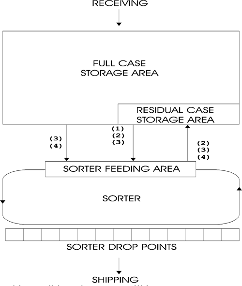
The residual carton has fewer than 10 units. For this condition, the carton will be sent to
the sorter and will not return to the residual area; however, a full-case carton must be sent to the sorter, partially emptied, and returned to the residual area.

No residual carton is available for that SKU. For this condition, no carton will come to the sorter from the residual area, a full-case carton will be sent to the sorter to be partially emptied, and that carton will return to the residual area.

For each condition with the exception of #4, a carton needs to come from the residual area to the sorter. The probability of #4 occurring is:

1 / (units per receiving carton) = 1 / 20

The probability of #4 not occurring is then 19 / 20. This is also the probability of one carton being sent from the residual-case area to the sorter per active SKU in the wave.
For each condition with the exception of #1, a carton must return to the residual area from the sorter. The probability of #1 occurring is 1 / 20. The probability of #1 not occurring is 19 / 20, which is also the probability of one carton returning to the residual area from the sorter per active SKU in the wave.

If a dual transaction is defined as one carton going from the residual area to the sorter and one carton going from the sorter to the residual area, the total number of dual carton transactions per wave can be calculated as follows:

In this example, the expected number of dual transactions per wave between the residual area and the sorter would be:

DualTransactions / Wave = (2,500)(1-(1/20))=2,375

Once the expected transactions between the residual area and the sorter have been determined, the expected transactions from the full-case area to the sorter must be calculated. To accomplish this, the flow into and out of the residual area must first be examined.

During normal operation, units are sent from the residual area to the sorter to complete orders (scenarios #1, #2, and #3), and other units, originally in full-case cartons, are sent to the residual area (scenarios #3 and #4). The net flow of units into and out of the residual area must be zero; otherwise, the residual area would be flooded or empty after some period of operation. If the net flow of units into and out of the residual area during a wave is zero, the total number of units sent to the sorter to complete orders has to come from the full-case area—not as the same SKU mix, but as the same total number of units. Therefore, the expected transactions between the full-case area and the sorter per wave are:

Given that the cartons sent from the full-case area to the sorter need to be replaced with new cartons sent from receiving to the full-case area, these transactions would also be dual transactions.

In this example, the expected dual transactions for the full-case area would be:

DualTransactions / Wave = (25,000)(1/20)=1,250

The total number of dual transactions per wave is the number of dual transactions for the residual area and dual transactions for the full-case area combined, or:

TotalDualTransactions / Wave = 2,375 + 1,250 = 3,625

For a series of four two-hour waves (eight hours per day divided by four waves per day), the required number of dual transactions per hour for the AS/RS is:

TotalDualTransactions / Hour = 3,625 / 2 = 1,813

Throughput Solutions

For an automated warehouse system consisting of a sorter and an AS/RS to feed the sorter, the required sorter drop points are:

Orders/Day
Waves/Day

and the AS/RS required dual transactions per hour are:

The distinction this example makes between full-case and residual storage areas illustrates their differences. The full-case area contains most of the distribution center’s inventory, but requires fewer transactions. The residual area, by comparison, has small storage requirements, but must facilitate a greater number of transactions. In other words, the full-case area has high storage requirements and low throughput requirements, while the residual-case area has high throughput requirements and low storage requirements.

Based on the preceding analysis, the full-case and residual storage areas clearly have different requirements that justify different recommended solutions. The money spent in the full-case area should focus more on efficient storage capacity and less on efficient/fancy throughput capabilities (i.e., conventional rack with manned vehicles). On the other hand, investment in the residual area should be directed at high and efficient throughput capabilities with less emphasis on storage efficiency (i.e., AS/RS, stackers, carrousels). The segregation of the storage area into residual and full-case areas does not present the problems that the segregation of fast and slow movers does. There is no need to define which SKUs are fast movers and which are slow movers, to re-evaluate categories periodically, or to move SKUs from one area to another as their status changes.

The change from a manual operation to an automated system forces decision makers to develop a new view of the warehouse and the factors driving it. Distribution center managers will achieve better results if the requirements for the entire operation are considered as a whole, rather than attempting to automate individual parts of a manual system.

Download PDF

In our industry (distribution) we are seen as primarily providing a “necessary” service to our organizations. We exist mostly out of necessity. More often than not, top management would like us to be “invisible”. They would like to have us deliver, without a hitch, whatever volume of product instantly and seamlessly. We need to deliver at a constant predictable cost—regardless of the volume. If you asked top management of companies that have distribution operations to list the “core competencies” of their organizations, it is doubtful that over 15% would include in the list “distribution services”. If you are one of the lucky ones whose organization views distribution as a “core competency” you have either done a great job and/or your management clearly understands the necessity of distribution and has provided equitable resources to make distribution core to the organization.

In nearly every financially “visible” change in distribution we are rightly asked to “cost justify” the change. The objectives of “changes in distribution” are normally related to: 1) increase in capacity, 2) increase productivity, or 3) reduction in the fulfillment time (life cycle). Capacity, productivity and fulfillment time have a unique relationship. The clarification of that relationship and its association with justification or return-on-investment (ROI) is the purpose of this paper. The paper primarily focuses on the “fulfillment” end of distribution rather than the “storage” or “inventory” end of distribution. The principles and techniques presented here are generally applicable to all distribution activities.

An increase in “capacity” in the context of this paper is defined as the ability of a distribution system to deliver more volume per time period. An increase in productivity is defined as an increase in the delivery of product per operational dollar. Capacity is delivery volume as a function of time; productivity is delivery volume as a function of cost. Many times the terms “capacity” and “productivity” are used synonymously. This is common because normally an increase in productivity yields an increase in capacity. However, an increase in productivity does NOT always yield and increase in capacity. Likewise, an increase in capacity can be achieved independently of an increase in productivity. A couple of examples are in order. Example 1: A completely manual system with one worker operating in a single area can achieve a capacity increase by adding an additional worker. The second worker, although adding to the total system capacity, reduces the efficiency of the first worker in the same, and now more congested, area. In this example a capacity increase yielded a productivity decrease. Example 2: A system where workers deliver product to a sorting system with insufficient capacity. The “operation” can be modified to increase productivity by immediately moving workers to another area once the shipping system backs up the work (rather than having them stand idle waiting for the sorter to clear out). This change can increase productivity (by using previously unused worker idle time) but will not increase capacity. Example 3: Carrying example 2 further, the “system change” in moving an idle worker does not move the resource back until the shipping sorter is completely cleared out. This change, while increasing productivity, would reduce system capacity by have the shipping sorter idle for a period of time.

Here are two basic rules concerning capacity and productivity increases. 1) A beneficial capacity increase will yield a greater delivery volume as long as the change is accompanied by consumption of additional resources that are proportionally less than or equal to the increased capacity. 2) A beneficial productivity increase is one, which yields a greater efficiency in the use of a resource and does not decrease capacity.

A quick note on fulfillment time or fulfillment life cycle: Although fulfillment life cycle is certainly effected by both productivity and capacity, the life cycle is more a function of the amount of work in-process in the facility. To reduce the fulfillment life cycle a focus must be made to reduce the work in process. Merely prioritizing work, while reducing some fulfillment times will increase others. The net effect of which (prioritization of specific fulfillment requirements) is normally a reduction in the overall productivity and capacity.

Beneficial fulfillment time reductions are usually associated with a reduction in WIP and do not adversely affect either productivity or capacity. Fulfillment life cycle improvements are normally justified by changing business requirements or by space utilization reduction.

Now to the meat of the discussion, how are change requests justified. Change requests for productivity are normally justified by a reduction in the cost of the operation. Productivity is a function of dollars. Such changes may also result in an increase in capacity and that benefit may be additional in-direct justification.

Capacity itself is not a function of cost; it is a function of time. The old saying “time is money” may be true but what is the equation? Justification for changes (increases in) capacity must be evaluated using a different technique. Capacity increases are justified in terms of identifying the alternatives. For example, how does a company “justify” the building their initial “distribution system”? If they do not build it they are not able to deliver product and they are not a company! That is all the justification it takes—the alternative! It is “justifiable” in some cases that adding capacity will actually reduce productivity. This situation is found many times in very seasonal businesses. In these cases, during peak season, additional less efficient resources are used to increase the capacity. This is justified by the alternative of adding capacity through additional capital expenditure that is not needed for a large part of the year.

Pretty simple, the hard part in justifying capacity increases is the willingness to take the effort to identify the cost of the alternatives!

Download PDF

Distribution centers often increase the productivity of labor-intensive piece-picking operations by clustering (or batching) multiple orders and picking them together. As the number of clustered orders increases, pickers become more productive because they spend less time walking between picks. The size of these order batches can be greatly increased through the use of a secondary sort using devices such as a tilt tray or Bombay sorter.

Sorter-based operations cluster orders using two different kinds of processes: Batch processing and continuous processing. This paper describes the differences between the two processes.

Application Example

The application case to be presented in this paper is a distribution center servicing a retail chain of 3,000 stores. Replenishment orders are available daily from store’s cash registers. Replenishment to the retail chain stores is mainly in less than full-case quantities (eaches or pieces). The distribution center operation uses a tilt tray sorter with 1,000 chutes. Each chute is assigned to a particular store for the duration of the fulfillment of that store replenishment order. Items are picked using printed pick lists and delivered to the sorter in pallets, cases or as individual pieces to fill the 1,000 clustered orders.

Batch Processing and “Waves”

The most common way to operate sorter-based systems is to create batches or waves. The work is organized in waves where:

Wave Orders = Number of Sorter Chutes

Day Waves = Day Orders / Wave Orders

In this type of operation waves are very well differentiated. The next wave may not start processing until the previous wave is completed. In theory, the number of clustered orders is equal to the number of sorter chutes; however, as a wave approaches completion, individual orders start completing and the actual number of clustered orders decreases.

Straggler items are a major problem in batch processes. As the next wave cannot start until the previous wave completes, a large number of pickers could be idle waiting for the stragglers of the previous wave to reach the sorter. While sorter utilization can reach almost 100% during the sorting of the initial portion of the wave, during wave transitions the utilization can drop to almost zero. This situation is like the old elementary school math problem asking for a solution of how fast a car must travel to make an average speed of 60 miles per hour over a distance of 30 miles if during our journey we stop for 15 minutes for a break.

The net effect of wave transitions can reduce the effective utilization of the sorter to 60% or 70%. With a device as expensive as a piece sorter such a low utilization is a serious problem.

Batch Processing Implementation—living with wave transition

In this example, daily delivery to each of the 3,000 stores requires that the sorter operate with at least 3 waves since the number of stores is 3 times the number of sorter chutes. To minimize the effect of wave transitions it may be possible to create queues where work continues during transitions or to organize work such that staff is either reduced or re-assigned to other functions during idle times. Minimization efforts of the effects of wave transition are normally accompanied with double handling and inefficiencies of their own. In the end, wave transition low sorter utilization is normally accepted as just a “fact of life”.

Batch Processing Implementation—living with limited sorter chutes

Many sorter systems were initially designed to have a sufficient number of chutes to allow all daily orders to be picked in one single batch. Although this method did not eliminate the wave transitions, staff could be released as the daily work subsided leaving only a reduced staff to deal with handling the end of wave stragglers. This situation works perfectly in situations where there are a sufficient number of available chutes. However, in our example, since the number of stores is three times the number of chutes, the use of this solution requires limiting the delivery to only 1,000 stores daily. The stores receive a delivery once each three days. This method eliminates the issue of low sorter utilization, but accepts limited delivery cycles as a “fact of life”.

Continuous Processing Implementation

• There is a permanent pool of orders (stores) pending to be processed.
• Orders can be pulled from stores as often as needed. Pulled orders are added to the existing orders in the order pool.
• There is a circular list of stores indicating the sequence in which orders are processed.
• The sorter processes 1,000 stores simultaneously. Every time that a chute is freed the current order for the next store in the list is assigned to that chute.
• Every time that a store is assigned to a chute, inventory allocation is re-calculated.
• Every time that a picker drops product (pallet, cases, or pieces) a new pick list is printed in real-time based on the last inventory allocation. If picking zones are falling behind the other zones, the software identifies the unbalancing and relocates pickers to correct the problem.
• All 3,000 stores can be serviced every day.

The main difference between continuous and batch processing is the absence of waves in a continuous process. In a continuous process as soon as an order completes and frees its chute a new order is assigned to the chute. This means that in a continuous process the number of clustered orders is always equal to the number of sorter chutes.

Straggler items do not go away in a continuous process. However, a continuous process can handle stragglers a lot better than a batch process. In a continuous process, straggler items only affect the orders they belong to and the chutes where those orders are assigned, while the other chutes can continue working without any interruption. Pickers never become idle waiting for other pickers to catch up with them. A smooth continuous process should allow the sorter utilization to reach a steady-state utilization close to 100%, allowing the distribution center to maximize the benefit of the device and its investment.

Conclusion

Distribution centers have used piece sorters to cluster large number of orders for a long time. When the practice started, pickers used pick lists printed in batches long before the actual transactions were executed, dynamic allocation of sorter chutes was not feasible, and inventory allocation for orders could not be executed in real-time as transactions were executed. Batch processing should be considered a remaining trace from those old times.

Continuous processing is far superior to batch processing. With today’s existing resources there is no need to continue using batch processing. Low productivity wave transition times can be eliminated, idle workers waiting for others to catch up can become productive, customers (stores in our example) can be serviced better.

Download PDF

Batch picking orders is an efficient way to reduce walking in a distribution center. Piece sorters (tilt tray, cross belt, bombay) allow maximizing the number of orders to pick as a batch. Unfortunately, piece sorters are very expensive devices. The larger the number of orders to batch with a piece sorter, the longer the sorter has to be, and the more expensive it gets.

Double sortation is an approach that allows piece sorters to increase the number of orders to batch without requiring the single sortation length.

Conventional Double Sort Process

Sorter prices have a strong linear dependency on the sorter length. The chute section of a sorter is normally its longest section.

In a conventional single sort process, a sorter chute is required for each order in the batch to pick. A system designed for 1,000-order batches needs to have 1,000 chutes. At 3 ft. of sorter for each couple of chutes, the chute section of the sorter is 1,500 ft. long.

If a double sort process were used items are first sorted into waves and the then each wave is sorted into orders. The total number of sorter destinations could be reduced to as few as 68: 34 for the initial wave sort and 34 for the secondary order sort. There are other configurations of sorter destinations; however, the closer the primary and secondary sorts have equal number of destinations the fewer total sorter destinations are required.

Let us consider a system for 10 waves of 100 orders each, not as optimum as the one with the 34/34 configuration, but easier to visualize. The sorter needs 100 order chutes and 10 wave chutes. If wave chutes were 5 ft. of sorter for each couple of chutes, the chute section of the sorter would be only 175 ft. So, for the same number of orders to pick as a batch, the required chute section of the sorter using double sortation is less than 12% of the chute section using single sortation.

Normally the 1,000 orders are picked together are called a pick wave, their section of the sorter is called wave sorter. The 100 orders sorted together by the presort process are called a pack wave and their sorter section is called order sorter.

The extra handling of items required in a double sort process is easily justified with the savings on the sorter cost. However, the number of waves to process is rather large. In a traditional sorter process with static waves (next wave does not start until previous wave is fully completed) the inefficient wave transition periods can add up to large reductions in capacity and productivity with long periods of empty trays and idle inductors. What’s more, the transition period is largely independent of the actual size of the pick wave. Small pick waves take nearly the same time to finish the final few units, as do large pick waves.

Continuous Double Sort Process

The ideal solution for wave transition issues is a waveless process. Instead of static pick waves, the system can keep adding dynamically batches of 100 orders to the pickers’ tasks as wave sorter chutes are completing. The new orders are sorted to the chute that just completed. Pickers and inductors do not need to wait at the end of a pick wave for the next wave to start. The long periods with empty sorter trays are eliminated. Picking batches are larger as pickers are continuously picking for 1,000 orders. Utilizing the idle times of the sorter and the workers can increase capacity/productivity by up to 30%.

Real-time RF-directed picking is the best scenario for implementing waveless picking processes. In applications that require labeling of the sorted items, RF picking is still feasible if the label can be done at the packing stations.

Quasi-Continuous Double Sort Process

Due to labeling requirements, some applications do not allow the implementation of a complete waveless process. However, if label generation is dynamic and is printed at multiple stations along the pick path and completed pick assignments can be dropped off at these points a quasi-continuous waveless process is possible.

Some operations may require well defined pick waves and dynamically created pack waves are not an option. Such operations can also have continuous waveless presort operations by utilizing only half of the wave sorter destinations for each pick wave. Wave sort uses alternate destinations every other pick wave. The negative effect of this approach is the reduction of the pick wave size by half. Often, people try to alleviate this disadvantage using more than half of the chutes, hoping that some of them will be completed by the start of the next wave. The mathematics of probability quickly dispels any such hope.

In most operations there is flexibility regarding specifically what orders go to each pack wave. Taking advantage of software that supports dynamic chute allocation, it is possible to create a continuous presort operation where there are no wave transition periods and where pick waves actually have a proportionally longer time to complete. This technique takes advantage of the fact that not all the wave sort destinations are required from the beginning of a new pick wave.

Continuous waveless processing of the order sort process is also possible using similar techniques through the use of dynamic optimization. Double sort operations may be truly become waveless operations.

Conclusion

Double sort processing is an excellent approach to get the benefits of large picking batches without having to pay the full price of the required sortation equipment to support it. Double sort processing can be enhanced further with software that can support non-conventional operations.